FCN은 Fully Convolutional Networks for Semtantic Segmenation이란 논문에서 나온 컴퓨터 비전 알고리즘이다. (링크)
저자는 Jonathan Long, Evan Shelhamer, Trevor Darrell 이다.
제목에서도 알 수 있듯이 Semantic Segmentation 분야의 문제를 풀고자 하는 논문이다.
Abstract
본 논문은 Semantic segmentation의 최신 성능을 능가했다. 핵심적인 통찰 중 하나는 'fully convolutional' network로 이를 통해서 arbitrary size, 어떠한 사이즈라도 상관 없이 input을 받아서 그에 따른 사이즈의 output을 반환하면서 동시에 학습과 추론에 있어서도 효율적이다. AlexNet, VGG net, GoogLeNet을 적용하였다. 또한 skip architecrue를 정의하고 이를 deep coarse layer의 semantic information과 결합하였다. PASCAL VOC, NYUDv2, 그리고 SIFT Flow에 대해서 SOTA 결과를 달성하였으며 추론에 있어서 0.2초 (one fifth of a second)보다 적은 시간이 걸렸다.
1. Introduction
FCN (Fully Convolutional Networks)은 end-to-end와 pixels-to-pixels로 학습했으며 SOTA 성능을 달성했다.
FCN은 효율적이며 다른 작업들과 다르게 복잡함을 배제한다.
Semantic segmentation은 semantics과 location 사이의 긴장 상태에 직면해있다. Global information은 what, 무엇인지에 대한 문제를 해결하며 동시에 local information은 where 어디에 있는지에 대한 문제를 해결한다.
Deep feature hierarchies는 location과 semantics 정보를 비선형적인 local-to-global 피라미드로 표현(encode)한다.
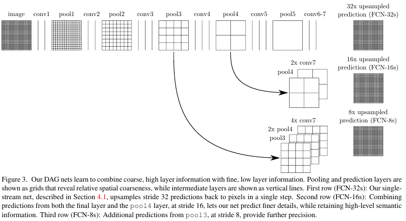
저자들은 skip architecure를 통하여 deep, coarse, semantic 정보와 shallow, fine, appearance 정보를 혼합하여 피쳐들의 스펙트럼에 따른 이점을 가져간다.
3. Fully convolutional networks
Convnets는 translation invariance에 기초한다. Convolution, pooling, activation functions에 의해서 Convnets는 오직 relative spatial coordinates 상대적인 공간 정보에만 의존하여 학습한다. 따라서 어떠한 사이즈라도 상관없이 input을 받아서 처리할 수 있다.

3.1. Adapting classifiers for dense predicton
기존의 Classification까지 이어지던 작업을 Figure 2에 나온 것 처럼 수정해서 heatmap을 리턴하도록 응용한다.
이때 semantic segmentation은 input size와 같은 개수의 pixels를 예측하므로 dense prediction 문제라고 할 수 있다.
3.2. Shift-and-stitch is filter rarefaction
Dense prediction은 coarse outputs를 stitch 봉합하여 input의 shifted version으로 볼 수 있는 output을 만들 수 있다.
Output이 factor f에 의해 downsample 되었다면 f2만큼 upsampling한다.
conv layer의 filter weight가 fij이고 stride가 s라면, Upsample은 아래와 같이 이루어진다.
이를 논문에서는 rarefy the filter by enlarging이라고 한다.
f′ij=fi/s,j/s if s divides both i and j.
하지만 위와 같은 방법은 사용하지 않았다.
3.3. Upsampling is backwards strided convolution
또 다른 방법은 바로 interpolation이다. 하지만 이를 사용하지 않는데 그 이유는 backwards convolution (또는 deconvolution) with an with an output stride of f 이 업샘플링 방법이기 때문이다. Factor가 f인 upsampling이 곧 fractional input with stride of 1/f인 convolution이다.
구체적인 deconvolution의 그림은 아래과 같다. (출처)
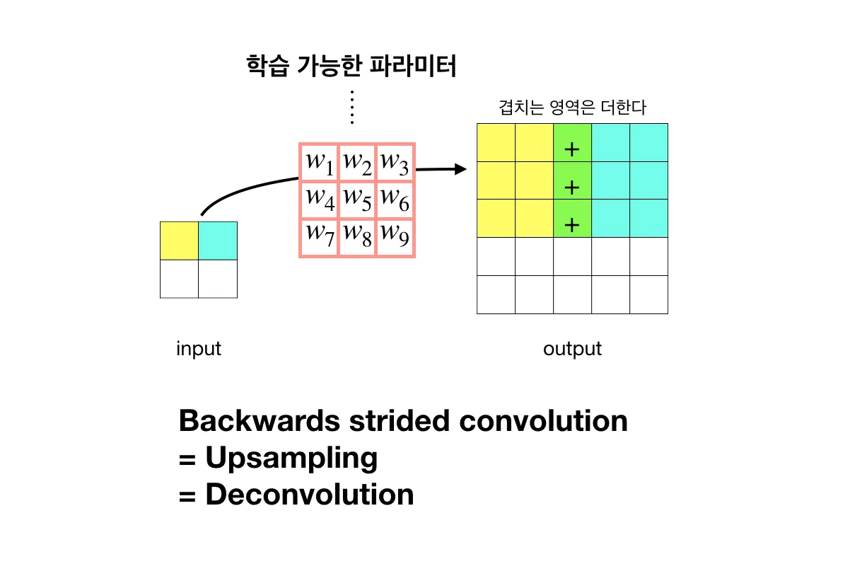
Convolution과 반대로 작동한다.
즉 Deconvolution은 위 노란색 칸이 c1이라고 할 때,
c1*w1 = output(1,1),
c1*w2 = output(1,2),
...
이런식으로 작동한다.
반면에 convolution은 다음과 같이 동작한다.
input(1,1)∗w1+input(1,2)∗w2+...+input(3,3)∗w9 = c1
구체적으로 그리고 써보면 더 쉽게 이해가 된다.
3.4 Patchwise training is loss sampling
전체 이미지가 아닌 patch 단위로 쪼개서 학습할 수도 있다.
패치를 쪼개서 학습하는 것은 전체 이미지의 학습과 차이점이 없지만 패치 단위로 학습한다면 불필요한 중복 학습이 있을 수 있다.
또한 샘플링도 수행해보았으나 학습의 속도나 성능의 면에서 더 좋지 않았다.
4. Segmantation Architecture
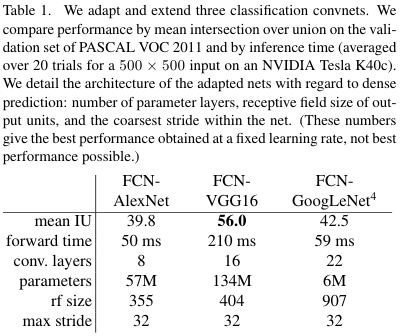
AlexNet, VGGNet, GoogLeNet을 백본 모델로 사용했다.
4.2. Combining what and where
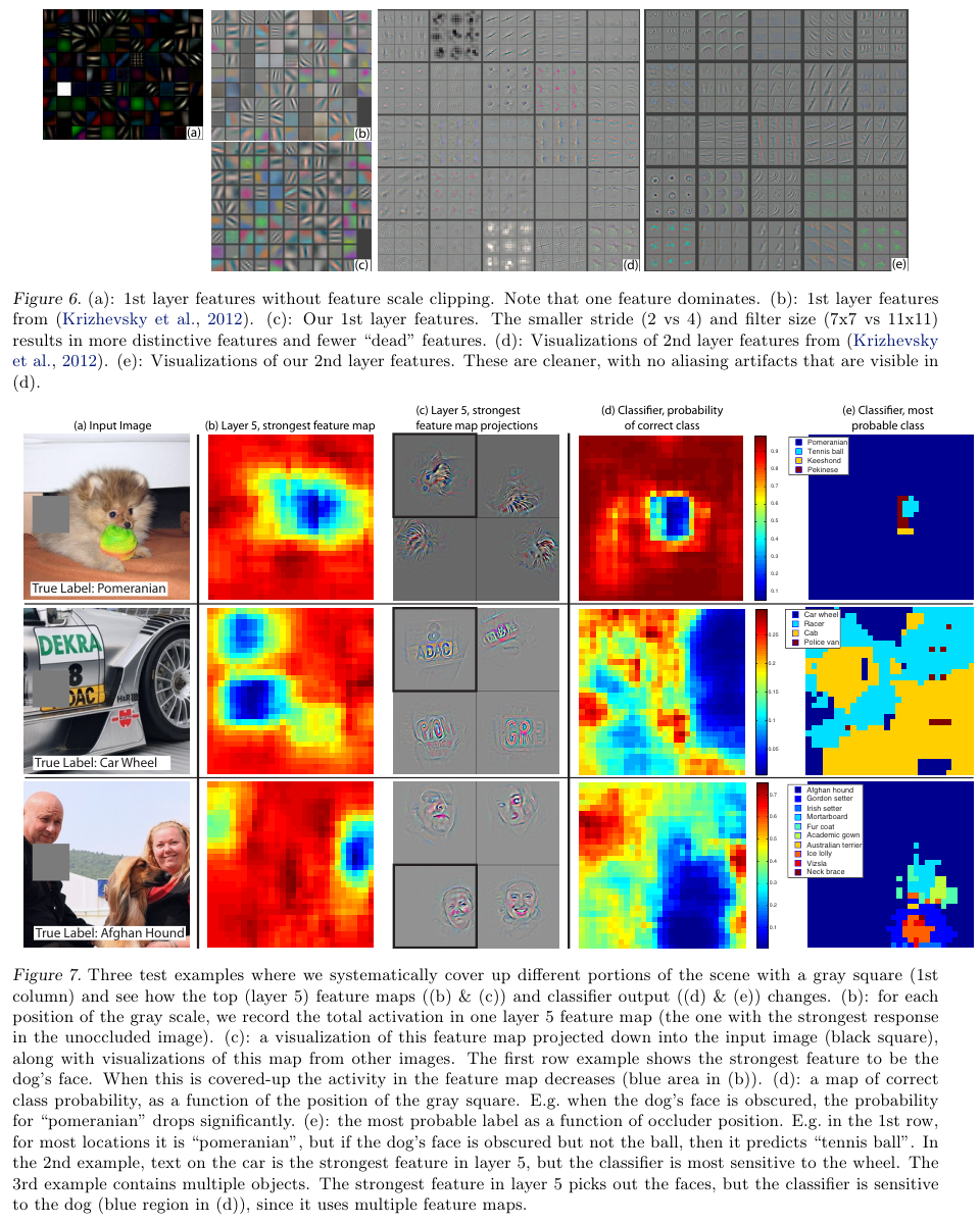
input에 가까운 shallow layer는 local feature를, 중간 layer는 coarse feature를, output에 가까운 deep layer는 global feature를 갖는다. (유명한 논문인 Visualizing and Understanding Convolutional Networks (링크) 에서 확인할 수 있다.)
Visualizing and Understanding Convolutional Networks의 Fig 6과 7을 아래 첨부했다.
Layer가 쌓일수록 보다 복잡한 feature를 학습했음을 알 수 있다.
따라서 저자들은 pool4에서 coarse feature를, pool3에서 상대적인 local feature를 가져와서 global and local feature를 모두 활용했다.
5. Results
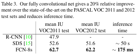
최종적으로 PASCAL VOC 2011과 2012의 test 결과를 볼 때 SOTA인 R-CNN과 SDS 보다 좋은 성능을 보이면서
추론 시간은 줄어들었음을 보인다.
References:
https://eremo2002.tistory.com/118
https://hwanny-yy.tistory.com/14
https://hyunseo-fullstackdiary.tistory.com/402
'Computer Vision' 카테고리의 다른 글
| U-net (2015) 논문 리뷰 (0) | 2025.04.06 |
|---|---|
| DeepLab v1(2016) 논문 리뷰 (0) | 2025.04.06 |
| Faster R-CNN (2016) 논문 리뷰 (0) | 2024.04.27 |
| ResNet (2016) 논문 리뷰 (0) | 2024.04.15 |
| Fast R-CNN (2015) 논문 리뷰 (0) | 2024.04.14 |


