Scaling Laws for Neural Language Models는 언어 모델에서의 데이터와 모델 사이즈를 늘리는 것에 대한 체계적인 연구를 다룬 논문이다. GPT-3에서도 언급되었으며 LLM의 중요한 기반이 되는 논문이다. (링크)
저자는 Jared Kaplan, Sam McCandlish, Tom Henighan, Tom B. Brown, Benjamin Chess, Rewon Child, Scott Gray, Alec Radford, Jeffrey Wu, Dario Amodei이다.
OpenAI에서 발표한 논문으로 LLM의 이론적 실험적인 증거가 되는 논문이다.
그전에는 결과만 보고 넘어갔는데 이번 기회에 다소 자세하게 논문을 살펴보고 이해해서 정리하고자 한자.
Abstract
크로스 엔트로피를 사용하는 Scaling law for LM에 대한 empirical 실증적인 연구다.
모델의 크기, 데이터셋의 크기, 그리고 학습에 사용되는 계산량을 간단한 Power law와 로그 스케일로 표기할 수 있다.
오버피팅과 모델/데이터 크기 그리고 학습 속도와 모델 크기를 간단한 방정식으로 나타낼 수 있다.
Summary
주요 결과의 요약이다.
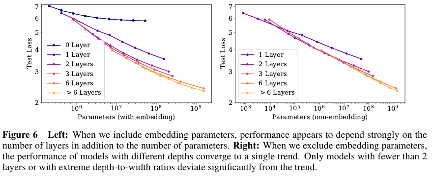
Performance depends strongly on scale, weakly on model shape:
모델의 성능은 대부분 다음의 세 가지에 강하게 달려있다. 바로 (임베딩을 제외한) 모델 파라미터 크기인 N, 데이터셋의 크기인 D, 학습에 사용된 연산량 C (amount of compute). 극단적인 경우를 제외하고 모델의 성능은 depth가 width과 같은 다른 구조에는 상대적으로 약하게 영향을 받는다. (Section 3)
Smooth power laws:
성능은 N, D, C 각각의 관계가 Power law (멱 법칙)을 따른다. 단 다른 두 가지 요소에 의해서 병목현상이 생기지 않는다는 전제가 필요하다. 6자리 이상의 (six orders of magnitude) 자리수에 대해 적용된다. (Section 3)
Universality of overfitting:
N과 D를 늘리면 성능은 향상되지만, 하나를 고정하고 다른 하나를 늘린다면 수확 체감의 법칙 (regime of diminishing returns)에 진입한다. $N^{0.74} / D$ 비율을 고려하여 오버피팅을 피할 수 있다. 이는 모델의 크기가 8배 증가할 때 (8x) 데이터가 약 5배 (5x) 증가하면 이를 피할 수 있다는 뜻이다. (Section 4)
Universality of training:
학습 곡선은 예산 가능한 Power laws를 따른다. Extrapolating (외삽법) 을 초기 학습 곡선에 도입함으로써 학습이 길어짐으로써 생기는 loss를 예측 가능하다. (Section 5)
Extrapolation (외삽법): 현재의 정보를 이용해 미래를 예측하거나 추정하는 것
Transfer improves with test performance:
학습 데이터와 다른 분포를 가진 텍스트로 모델을 평가할 때, 실험 결과는 학습에서 사용한 validation 검증 데이터에 대한 결과와 대략적으로 constant offset in loss 상수 로스 오프셋은 서로 강한 상관관계를 가진다. 다른 분포의 데이터로의 전이 학습은 패널티를 발생시키지만 그외의 경우에서는 학습 데이터에 대해서 성능 향상이 발생한다. (Section 3.2.2)
Sample efficiency:
큰 모델은 작은 모델보다 샘플 효율적이라서 같은 성능 수준을 더 적은 데이터와 더 작은 optimization steps에서 달성 가능하다. (Figure 2)와 (Figure 4).
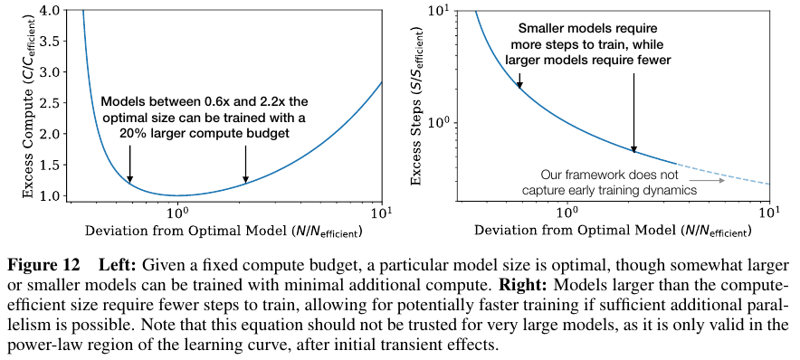
Convergence is inefficient:
연산량이 C로 고정일 때, N과 D에 제한이 없다면 매우 큰 모델 Very large model은 학습을 수행할 때 수렴하지 않음에도 early stopping을 적용함으로써 최적에 도달할 수 있다 (Figure 3).
따라서 실질적인 계산양 효율적인 학습은 예상 보다 더 빨리 도달 할 수 있다. 이는
최적화에 필요한 데이터의 양은 D ∼ $C^{0.27}$로 생각 보다 더 작다. (Section 6)
Optimal batch size:
최적의 배치 사이즈는 loss에 대한 Power law를 따르며 gradient noise scale을 측정함으로써 결정 가능하다.
저자들이 학습한 가장 큰 모델에 대해서 2 M tokens면 수렴 가능하다. (Section 5.1)

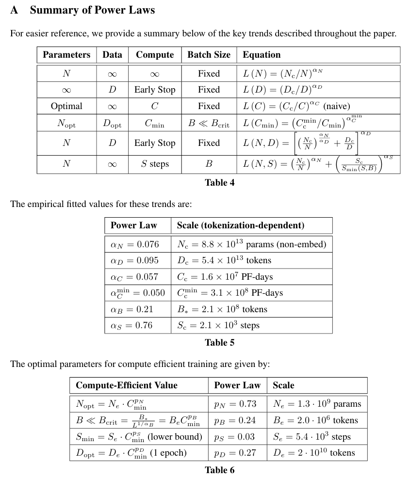
Summary of Power Laws
Powe laws의 식을 살펴 보기 전에 우선 노테이션을 정리하고 간다.
Notation
• L – the cross entropy loss in nats. Typically it will be averaged over the tokens in a context, but in some cases we report the loss for specific tokens within the context.
• N – the number of model parameters, excluding all vocabulary and positional embeddings
• B – Batch Size
• S – The number of training steps (i.e. parameter updates)
• C ≈ 6N BS – an estimate of the total non-embedding training compute.
We quote numerical values in PF-days, where one PF-day = 10 15 × 24 × 3600 = 8.64 × 10 19 floating point operations.
• D – the dataset size in tokens
• $\text{B}_\text{crit}$ the critical batch size, defined and discussed in Section 5.1. Training at the critical batch size provides a roughly optimal compromise between time and compute efficiency.
• $\text{C}_\text{min}$ – an estimate of the minimum amount of non-embedding compute to reach a given value of the loss. This is the training compute that would be used if the model were trained at a batch size much less than the critical batch size.
• $\text{S}_\text{min}$ – an estimate of the minimal number of training steps needed to reach a given value of the loss.
This is also the number of training steps that would be used if the model were trained at a batch size much greater than the critical batch size.
• $\alpha_\text{X}$ – power-law exponents for the scaling of the loss as L(X) ∝ 1/$\text{X}^{\alpha \text{X}}$ where X can be any of N, D, C, S, B, C min .
Equations
아래의 식들은 파라미터과 하이퍼파라미터들을 조정함으로써 Loss의 추이를 살펴본다.
그리고 이 Loss의 추이를 Figures에 나온 것과 동일하게 가져가기 위해서 모델의 크기, 데이터의 크기, 배치 사이즈 등을 어떻게 조정해야하는지를 탐구한다.
모델의 파라미터 수가 정해져있다면 필요한 데이터는 아래를 참고해서 계산해야 한다.
L(N) = $( N_c / N )^{\alpha_{N}}$, $\alpha_{N}$ ~ 0.076. $N_c$ ~ 8.8 x $10^{13}$ (non-embedding parameters) - (1.1)
데이터의 수가 정해져있다면 early stopping은 다음에 적용한다.
L(D) = $( D_c / D )^{\alpha_{D}}$, $\alpha_{D}$ ~ 0.095. $D_c$ ~ 5.4 x $10^13$ (tokens) - (1.2)
연산량이 정해져있고 충분히 큰 데이터가 준비되어 있고, 모델이 정해져있다면 필요한 배치 사이즈는,
$ L(\text{C}_\text{min}) $ = $( \text{C}_c^{\text{min}} / \text{C}_\text{min} )^{ \alpha_{C}^{\text{min}}}$, $ alpha_{C}^{\text{min}} $ ~ 0.050. $ \alpha_{C}^{\text{min}} $ ~ 3.1 x $10^8$ (PF-days) - (1.3)
Critical 배치 사이즈는 아래와 같이 정의된다. 크리티컬 배치 사이즈는 속도와 효율성의 트레이드 오프를 결정한다.
$ B_{\text{crit}}(L) = \frac{B_{*}}{L^{1 / { \alpha_{B} } }}$ , $B_{*}$ ~ 2 x $10^8$ tokens, $\alpha_B$ ~ 0.21 - (1.4)
L(N)와 L(D)를 동시에 적용한 다음의 식은 오버피팅의 정도를 결정한다.
L(N, D) = $ [ {(\frac{N_c}{N})}^{ \alpha_N / \alpha_D } + \frac{D_c}{D} ]^{\alpha_D} $ - (1.5)
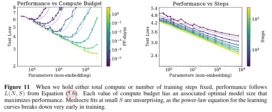
정해진 학습 스텝 S와 데이터의 수가 무한이라고 할 때 학습 곡선은 아래와 같다.
L(N, S) = $ {(\frac{N_c}{N})}^{ \alpha_N} + {( \frac{S_c}{S_{\text{min}} (S)} )}^{\alpha_S} $ - (1.6)
이때, $S_c \approx 2.1 \times 10^3, \alpha_S \approx 0.76$이다. $S_\text{min}(S)$는 가능한 모든 옵티마이제이션 스텝 중에서 최소값이다.
C가 정해져있을 때 식 (1.6)은 최적 모델 크기 N, 최적 배치 사이즈 B, 최적 학습 스텝 수 S, 데이터 사이즈 D를 계산할 수 있다.
N ∝$ C^{\alpha_{C}^{\text{min}} / \alpha_N}$, B ∝$ C^{\alpha_{C}^{\text{min}} / \alpha_B}$, S∝$ C^{\alpha_{C}^{\text{min}} / \alpha_S}, D = B \cdot S $ - (1.7)
$ \alpha_{C}^{\text{min}} = 1 / (1 / \alpha_S + 1 / \alpha_B + 1/ \alpha_N)$이다.
위 내용은 Appendix A에 정리되어 있는데 그 표들은 다음과 같다.
Parameters 수 세기

저자들은 GPT-2에서 사용했던 WebText의 확장 버젼인 WebText2와 BPE를 사용해서 학습을 했다고 한다.
이대 Vocab size는 50257이다. 1024-context token을 사용했다고 한다.
우선 $d_{attn}$ = $d_{model}$ = $d_{ff} / 4$다.
따라서 embed size는 ($n_{vocab}$ + $n_{ctx}$) $d_{model}$이다.
QKV multi head attention에서의 파라미터 수는 $n_{layer} \cdot d_{model} \cdot 3 d_{attn}$이다.
Q, K, V의 dim이 각각 $d_{attn}$ 이기 때문이다.
Attention-Project는 Multi-head attention을 수행한 결과를 다시 MLP를 수행한 결과다.
따라서 $n_{layer} \cdot d_{attn} \cdot d_{model}$ 만큼의 파라미터 개수가 필요하다.
Feedforard는 MLP를 2번 수행하므로 $n_{layer} \cdot 2 d_{model} \cdot 3 d_{ff}$다.
이를 모두 합하면 N이 된다.
N = $n_{layer} \cdot d_{model} \cdot 3 d_{attn} + n_{layer} \cdot d_{attn} \cdot d_{model} + n_{layer} \cdot 2 d_{model} \cdot 3 d_{ff}$
$\approx 12 \cdot n_{layer} \cdot {d_{model}}^2$다.
Experiments


전체 Figures 개수가 24개라서 일부만 가져왔다.
최적의 compute, dataset size, steps, model size를 이를 참조하면 도움이 많이 될것 같다.
References:
https://medium.com/nlplanet/two-minutes-nlp-scaling-laws-for-neural-language-models-add6061aece7
'NLP > LLM' 카테고리의 다른 글
| LaMDA (2022) 논문 리뷰 (0) | 2025.04.11 |
|---|---|
| PaLM (2022) 논문 리뷰 (0) | 2025.04.11 |
| LoRA (2021) 논문 리뷰 (0) | 2025.04.11 |
| OPT (2022) 논문 리뷰 (0) | 2025.04.11 |
| GPT 3 (2020) 논문 리뷰 (5) | 2025.04.09 |


